An Accelerator Model in SimPy, End to End

Topics We'll Cover

• What the Model Must Answer
• SimPy Primitives, Mapped to Hardware
• Back-Pressure in the Smallest Model
• From a Graph to Tiles
• The Timing Model: Cycle-Approximate Components
• Methods: Roofline, Little's Law, Utilisation and Bottlenecks
• Finding the Stalls
• Interactive: Where the Time Goes
• Real Models: Timeline and Hot-Spot
• Process-Based Against Cycle-Based
• How gem5 and SST Are Structured
• The Hot Path in C++ with pybind11
• Modern C++ in the Port
• ONNX Runtime Execution Providers
• An FHE Workload: Polynomial Products via the NTT
• Computing in the Data Path (Speculative)
• Specification, Tests and CI
• Reading List
• What to Take Away

What the Model Must Answer

Deck 10 turned PyTorch and ONNX models into operator traces and costed them on a roofline: one number per operator, no queues, no contention. An architect's next questions need time to pass: while the array computes, is the next tile already loading? Does the buffer fill? Which engine is everyone waiting for? This deck builds the event-driven model that answers them, simfront.accel in Torch_Sim_Frontend, and runs real graphs through it end to end.

Its one-page block specification (docs/accel_spec.md) is written as for a hardware block: contents, interfaces, behaviour, timing, ordering, counters and assumptions. Every number on these slides comes from examples/accel_results.md, and the two presets (edge-npu, dc-npu) are illustrative.

SimPy Primitives, Mapped to Hardware

SimPy has few primitives (InfSim 02 lists them all), and a data-movement accelerator needs only these:

def load_dma():
    for i, t in enumerate(tiles):
        tm.issue[i] = env.now
        o = first.get(i)
        if o is not None and o.deps:
            yield env.all_of([op_done[d] for d in o.deps])
        tm.dep[i] = env.now
        if t.alloc:
            yield buf.put(t.alloc)
        tm.alloc[i] = env.now
        if t.load_dur > 0:
            yield from transfer(t.load_dur, noc_r)
        tm.load_end[i] = env.now
        yield ready.put(i)

Back-Pressure in the Smallest Model

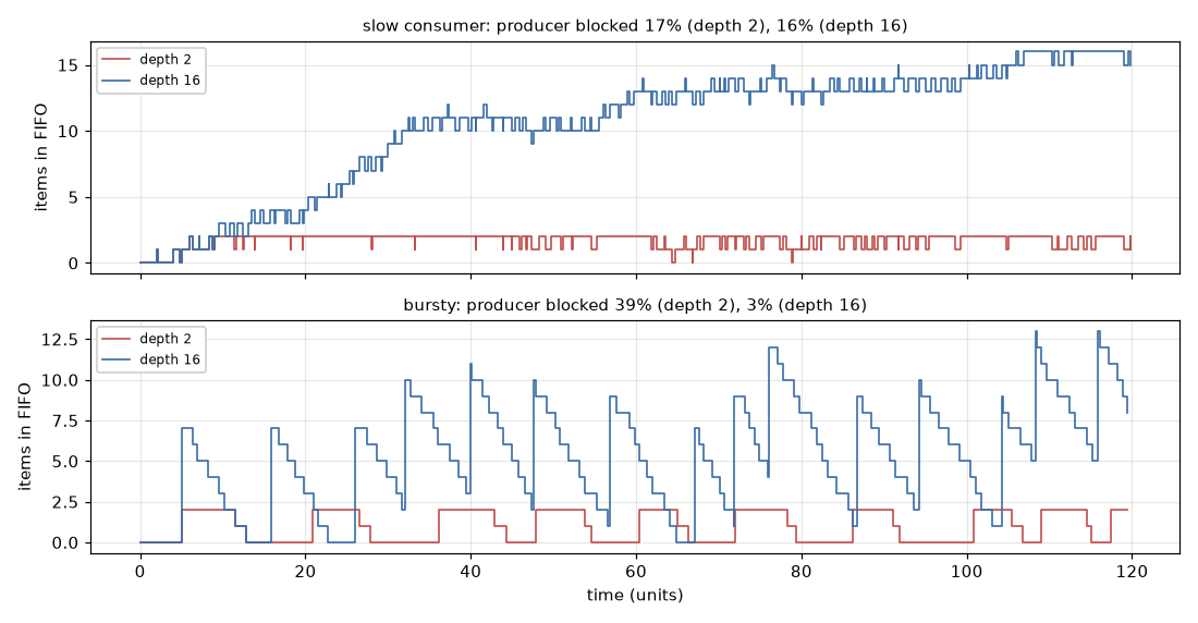
Before the accelerator, the property that matters most in it: a producer and a consumer joined by simpy.Store(capacity=depth). A full FIFO makes put wait, so a producer that runs ahead is stalled instead of filling an infinite queue. The probe records the depth at every change; fifo.py is the whole model.

Source: examples/accel_results.md in Torch_Sim_Frontend

Depth buys throughput only when the rates vary. With a consumer 20% slower, depth changes nothing (the consumer sets the rate). With bursty arrivals, going from depth 1 to 16 raises throughput from 0.5741 to 0.9641. Little's law (L = λW) holds exactly on every run, which the tests assert: a free check on the probes.

From a Graph to Tiles

The model takes a simfront-trace/1 trace from any of deck 10's front ends (torch.export, ONNX, the dispatch trace) and lowers it to tiles: the unit the hardware loads, computes and stores.

def _split_gemm(b: int, m: int, k: int, n: int, e_in: int, e_out: int, budget: int):
    """Block sizes (bb, bm, bk, bn) whose operands and result fit in ``budget`` bytes."""
    def size(bb, bm, bk, bn):
        return bb * (e_in * (bm * bk + bk * bn) + e_out * bm * bn)

    bm, bk, bn = m, k, n
    while size(1, bm, bk, bn) > budget:
        big = max(bm, bk, bn)
        if big == 1:
            raise ValueError(f"a 1x1x1 GEMM block does not fit in a {budget}-byte tile")
        if bm == big:
            bm = math.ceil(bm / 2)
        elif bn == big:
            bn = math.ceil(bn / 2)
        else:
            bk = math.ceil(bk / 2)
    bb = max(1, min(b, budget // size(1, bm, bk, bn))) if (bm, bk, bn) == (m, k, n) else 1
    return bb, bm, bk, bn

The same CNN exported by torch.export and by ONNX does the same 2,802,304 multiply-accumulates on the array by both routes (a test asserts it).

The Timing Model: Cycle-Approximate Components

Every duration is computed once, at lowering, so all three engines (the SimPy model, the fast path and the cycle-stepped twin) run the identical program.

Methods: Roofline, Little's Law, Utilisation and Bottlenecks

Four first-order methods that every simulator result should be checked against, and how this model uses each:

Latency against throughput. One inference's latency is the makespan; throughput needs the pipeline full. The FIFO slide is the throughput side of the same trade: depth (and buffer) buys throughput under variable rates, and costs latency and area (SimEng 13).

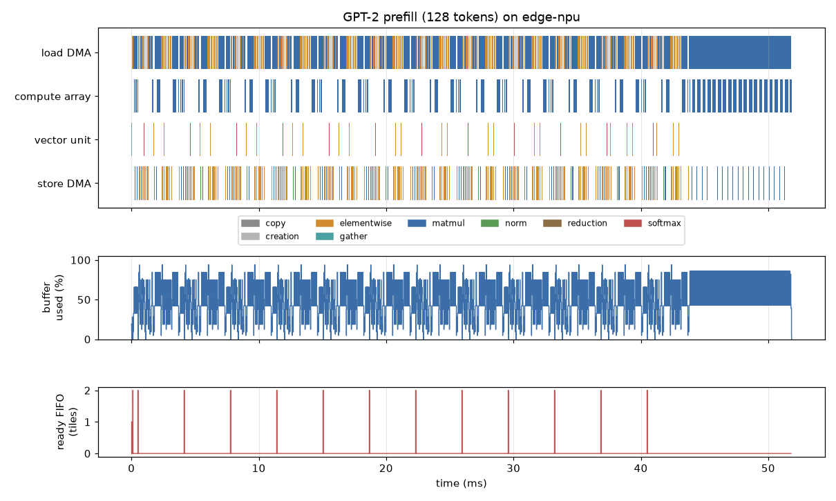
Utilisation is not saturation. GPT-2's prefill on edge-npu keeps the array at 31.0% (PE efficiency 98.1%) efficiency when busy, but busy only 31.0% of the run: the arithmetic is efficient, the array is starved.

Finding the Stalls

The compute units issue in order, so the run splits exactly into computing and the gaps between tiles. Each gap is attributed by walking back along the next tile's load: was it transferring (or the DMA still busy with earlier tiles: load bandwidth), waiting for buffer space (buffer full), or waiting for an earlier operator's results to be stored (dependency)? The parts sum to the latency on every run, a tested invariant.

Source: examples/accel_results.md in Torch_Sim_Frontend

For the small CNN on edge-npu, compute is 6.4% of the time; the hot-spot is off-chip memory, and the operator boundaries cost a third.

Interactive: Where the Time Goes

The recorded sweep (batch of eight images through the CNN, on the C++ fast path). Choose a configuration; the bar splits the compute units' time into computing and the three kinds of stall.

Real Models: Timeline and Hot-Spot

Published configurations, traced on the meta device without weights (deck 10), then simulated:

Source: examples/accel_results.md in Torch_Sim_Frontend

The timeline shows the hot-spot at a glance: the load DMA lane is nearly solid, the array lane is not. The last 8 ms is the LM-head matmul (50,257 × 768 weights): 15.5% of the run in one operator. Llama-3-8B on dc-npu is the opposite case: compute-bound, with the hot-spot on the array. The same intervals are written as a Chrome trace for Perfetto.

Process-Based Against Cycle-Based

An RTL simulator advances a clock and evaluates every block on every edge (Introduction to Simulation measures Icarus against Verilator). cycle.py does that to this accelerator: on every cycle each engine is a state machine that retires its tile if its countdown has expired and starts the next if it can. The SimPy model instead jumps from one state change to the next.

Source: examples/accel_results.md in Torch_Sim_Frontend

How gem5 and SST Are Structured

Two production simulators, built on the same three ideas as this model: components, connections with flow control, and an event queue. Names below are as in recent releases of each; their documentation (gem5, SST) is the reference.

The lesson for a model of this size: make the connection the unit of flow control, as both do. Here a Container is the port's ready signal; in gem5 it is a retry, in SST a credit. Parallel discrete-event simulation (InfSim 08) needs the lookahead that SST's link latencies provide.

The Hot Path in C++ with pybind11

The SimPy model spends its time on event bookkeeping: 20,775 events for GPT-2's 1051 tiles (slide 10), each a heap push and pop and a generator resumed (measure before porting: SimEng 11). When the two DMA engines cannot contend for a memory channel, the loop has nothing left to arbitrate, and every tile's times follow from earlier tiles': a recurrence with a min-heap of buffer frees. It is written in Python, then ported line for line to C++20 and exposed with pybind11. All three agree bit for bit on every field of every tile, on real traces and on Hypothesis-generated programs.

Source: examples/accel_results.md in Torch_Sim_Frontend

Modern C++ in the Port

The port is small, and uses the features worth knowing (SimEng 03 covers value types and RAII):

template <typename K>
concept Ordered = requires(const K& a, const K& b) {
    { a < b } -> std::convertible_to<bool>;
};

// A binary min-heap ordered by key(item). std::priority_queue would do; writing it out keeps
// the pop order identical to Python's heapq for equal keys (both break ties by a sequence number).
template <typename T, Ordered K, K (*key)(const T&)>
class MinHeap {

auto p = std::make_unique<Pipeline>(std::move(op), std::move(first), std::move(last), std::move(stores),
                                    std::move(alloc_in), std::move(alloc_out), std::move(load_dur),
                                    std::move(comp_dur), std::move(store_dur), std::move(deps), n_ops,
                                    capacity);
py::gil_scoped_release release;
return p->run();

• Templates and concepts. MinHeap<T, K, key> is a generic binary heap; the C++20 concept Ordered rejects a key type without < at compile time, with a readable error.
• Move semantics. The constructor takes each column by value and std::moves it into the object; run() moves its result columns out. No million-element vector is copied.
• Smart pointers. std::make_unique builds the pipeline; Python owns bound objects through std::unique_ptr, pybind11's default holder, so memory is freed when the Python object goes.
• std::span views a dependency list without copying; [[nodiscard]] and noexcept document intent.
• The GIL is released while the kernel runs, so Python threads can run sweeps in parallel.
• Same operation order as Python, so the doubles are identical (the parity checklist).

ONNX Runtime Execution Providers

A hardware backend joins ONNX Runtime as an execution provider (EP). When a session is created, ONNX Runtime asks each EP in priority order which nodes it can run (GetCapability), fuses each EP's connected nodes into subgraphs, and gives everything unclaimed to the CPU EP (InfSim 09; ORT: adding an EP). A real EP is C++ against ONNX Runtime; ep.py reproduces the partition so the simulator can cost it:

• ep.ort_providers runs a real session with profiling on and reads which provider ran each node;
• ep.claim is a GetCapability: claim by operator type, group connected claimed nodes;
• ep.simulate: claimed operators on the accelerator model, the rest on a host roofline, a link transfer for every crossing.

Source: examples/accel_results.md in Torch_Sim_Frontend

With these illustrative numbers the host is better at memory-bound operators than the edge device, so claiming fewer nodes is faster. The partition has to be costed, not counted: the point of operator coverage as a time metric.

An FHE Workload: Polynomial Products via the NTT

Lattice-based homomorphic encryption multiplies polynomials in Z_q[X]/(X^N+1), stored as one row of N residues per RNS prime ("limb"), through the NTT: c = INTT(NTT(a) · NTT(b)) after a twist by a 2N-th root of unity (FHESim 01). ntt.py has the golden model, checked against schoolbook multiplication by Hypothesis, and a workload builder in the same trace format, so it runs through the same accelerator.

def polymul(a: list[int], b: list[int], q: int) -> list[int]:
    """a * b in Z_q[X]/(X^n + 1) through the NTT (negacyclic twist by psi)."""
    n = len(a)
    p = psi(n, q)
    w = p * p % q
    tw = [pow(p, i, q) for i in range(n)]
    fa = ntt([x * t % q for x, t in zip(a, tw, strict=True)], q, w)
    fb = ntt([x * t % q for x, t in zip(b, tw, strict=True)], q, w)
    c = intt([x * y % q for x, y in zip(fa, fb, strict=True)], q, w)
    inv = pow(p, q - 2, q)
    return [x * pow(inv, i, q) % q for i, x in enumerate(c)]

One product at N = 2¹⁶ with 24 limbs is 96 operators. An NTT is (N/2) log₂N butterflies; at three operations each that is 3.0 operations per input byte. On dc-npu it takes 489.10 µs and is memory-bound; with a 16-lane vector unit, 2,789.18 µs and NTT-bound. The full FHE picture (key switching, bootstrapping, key traffic) is in FHESim 02 and FHE_Accelerator_Sim.

Computing in the Data Path (Speculative)

FHE is bound by data movement (FHESim 02), so one family of ideas moves the computation to the data: into memory (FHEmem, arXiv:2311.16293; APACHE, arXiv:2404.15819), into the network (in-network aggregation for training, SwitchML, arXiv:1903.06701), or onto light (FHESim 04, FOptInf 03). The model adds a stage in the memory read path that performs the NTT as the data streams in (a pipelined NTT, like the delay-feedback designs in Cryptography 10), with a budget in operations per byte.

Source: examples/accel_results.md in Torch_Sim_Frontend

Specification, Tests and CI

The model is held to the same discipline as the front end (SimEng 09): requirements SF-18 to SF-28 in EARS patterns, each traced to the tests that verify it by a matrix generated from the test run.

GitHub Actions runs the suite on Python 3.10 and 3.12 with SIMFRONT_REQUIRE_CPP=1, which turns a C++ module that failed to build into a test failure instead of a silent fallback to Python, then smoke-tests the CLI on the CNN, the NTT workload and the cycle-stepped twin.

Reading List

What to Take Away

• Four SimPy primitives model a data-movement accelerator: Resource for channels and links, Container for buffer bytes (back-pressure for free), Store for FIFOs, events for dependencies.
• Lower once, run many engines: the SimPy model, a bit-identical fast path (Python and C++), and a cycle-stepped twin that agrees cycle for cycle at a hundredfold cost.
• Find the stalls by attributing every gap, not by reading utilisation: a busy array can be starved, and a bigger buffer can be slower.
• gem5 and SST are built on the same three ideas: components, connections that carry flow control, and an event queue.
• Port after profiling, and measure the whole call: the algorithm bought more than the language, and conversion and lowering decide the end-to-end gain.
• An execution-provider partition, an in-transit stage or a new engine is a design decision only once it is costed in time.